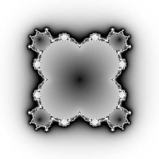
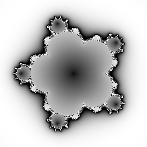
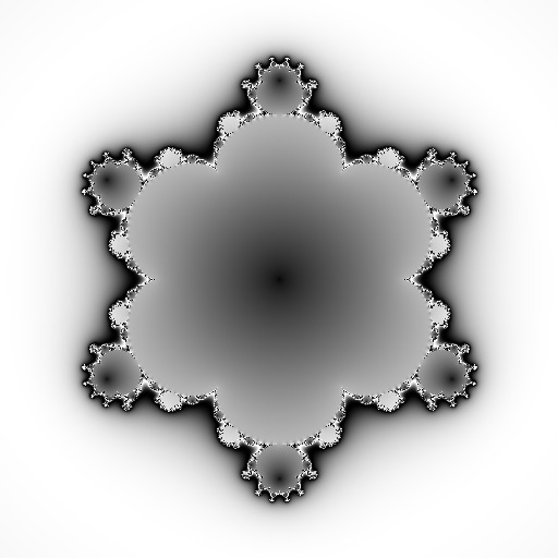
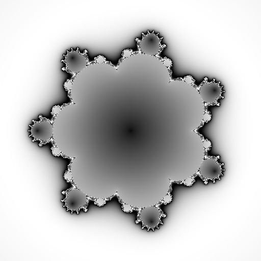
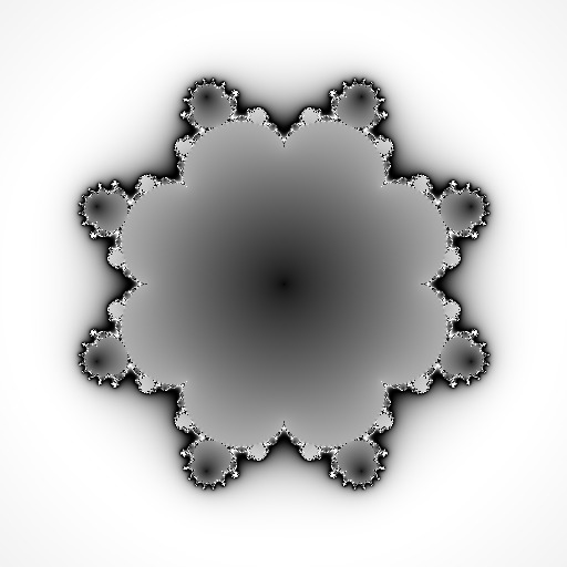
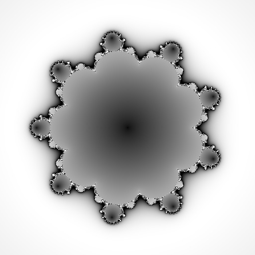
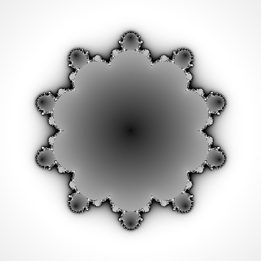
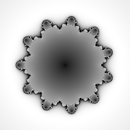
Getting to see the colourfully curvy parts of the complex space is a matter of degrees, positioning and technique - after all, the well-known 2nd degree polynomial can only get you round and round that same old mandelbrot island that turns forever and ad nauseam into itself. So, as a first step, just crank up your polynomial's degree while keeping just the top coefficient to 1 and the rest to 0. Then watch the mandelbrot multiply - split and split again, forever content to retrace that shape even in multiples. Here's how it looks, with black and white illustrations, why not:

When tired of all that perfect symmetry, whacking the coordinates one over the head with a well chosen function can do at least a bit of pleasing damage to the perfect mandelbrotian order but there's little gain in such a cheap trick - basically you're just looking at the same perfect symmetry only through a distorted lens, trying to pretend that if you marred your vision then the thing you're looking at has therefore changed as well. Even lying to oneself has got to be at least more fun than such sad attempt. So let the coordinates alone and the vision undisturbed but inject instead some controlled chaos by using a mersenne twister (MT) as a generator of more interesting complex polynomials: simply set all coefficients of the polynomial to the sequence obtained from the MT - all of a sudden, there's literally an infinity of polynomials of the same degree even¹ and the mandelbrotian order is left behind on the shores of piddly quadratic polynomials with boring 1 or 0 coefficients, while the space opens up and looks rather... empty perhaps:

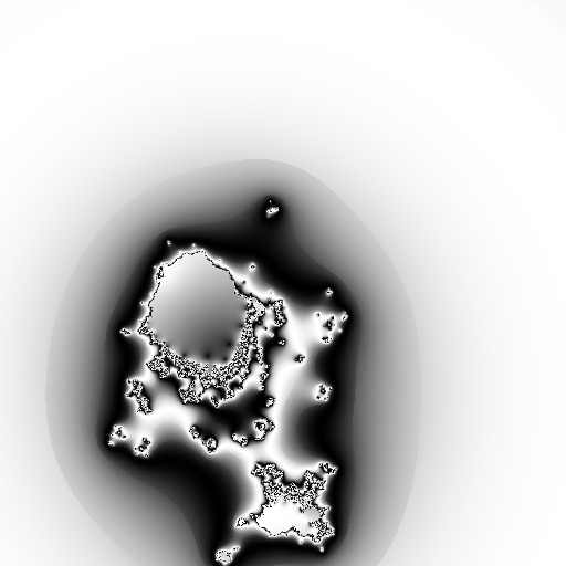
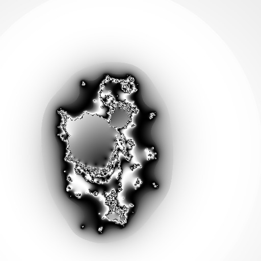
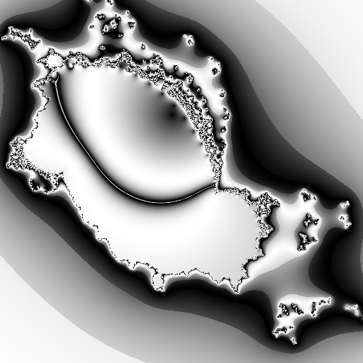
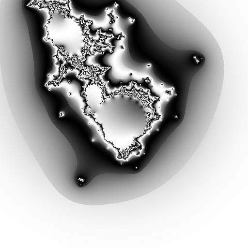
The above apparent emptiness of the space is of course just a matter of positioning: while the complex space is infinite, some parts of it can turn out - when seen through some of those polynomials and especially when not iterated too much² - infinitely boring and so best avoided. On the brighter side though, for all the infinity of the space (boring or otherwise), one can always map any portion of it wherever desired, so that there is no need to keep fiddling forever with the positioning or (even worse!) end up adjusting the positioning to something else for each new function. So one area is fine enough but which area might that be? Well, there is some pleasing symmetry around the origin, not to mention the fact that I haven't thrown out with the bath water the critical orbit too and that's still around (0,0). So pick some space around the origin³, adjust the zoom for more or less detail depending on whether you want basically small islands on the sea or something closer to mainland and fire up your pseudo-random number generators of the mersenne twister sort. Recall though that there was technique involved too if you are to get anywhere, so don't despair just yet if it still doesn't look all that curvy - or even interesting at all - when plotting just that old smoothed iteration count:

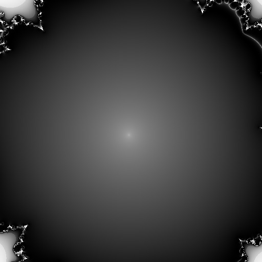
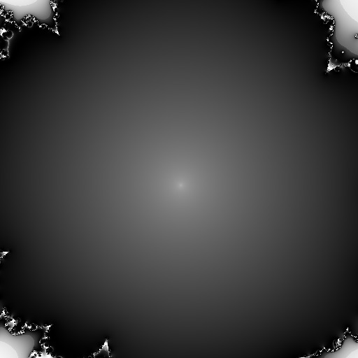
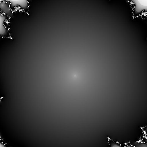
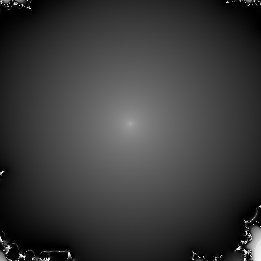
Having set as above the polynomial to use and the bit of space to look at, the last and by far more spectacular part is choosing what exactly to show of it and then how to colour-code it to produce the final image. Since I already had the average curvature colouring implemented, I gave that a spin, with the same trig-based grayscale formula for colour choice. Being an average curvature as opposed to a bland iteration count, it might be rather unsurprising that the result is quite curvy essentially - combined with the grayscale colour choice that curves and blends as well, one might perhaps find those white lines as not-bad mountain-range peaks sneaking their way around, on ever changing (if always rounded) directions of sorts:

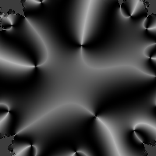
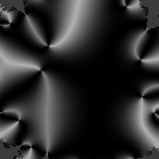
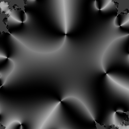
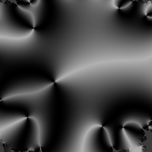
The above samples are really just that - samples of an infinite series, since each MT sequence results in a different "landscape" even if one of the same overall type otherwise. Still, since I rather like those curves in there, I really wanted to see them coloured up beyond this black & white that is meant for heightmaps - after all, whether this type of images make good heightmaps or not, they might still make interesting textures perhaps, if nicely coloured in. So I tweaked my formula for the black and white colouring to expand it to some pleasing walk through the r,g,b space⁴ and look what came out of it:

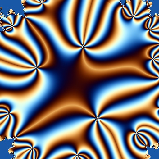
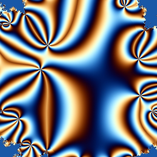
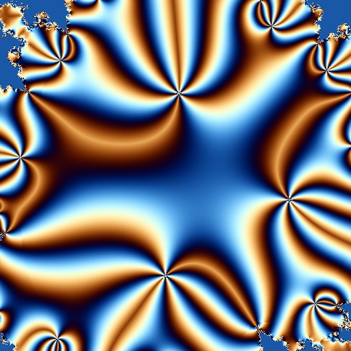
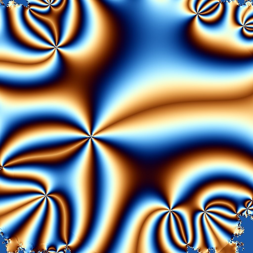
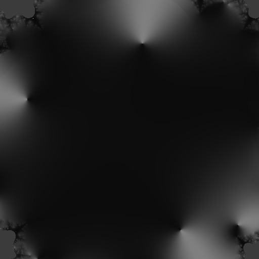
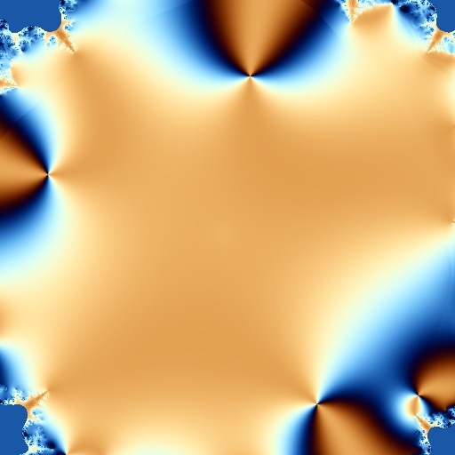
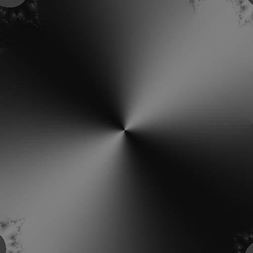
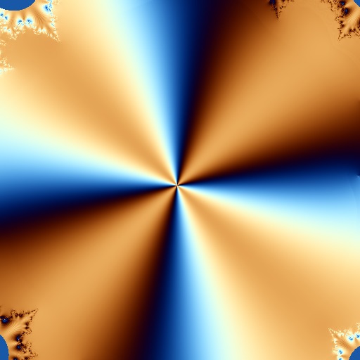
For completeness, I implemented as well two more averaging colouring techniques, namely the TIA (triangle inequality average) and the SA (stripes average). Neither of those seems to me very good for this exact series but they might come in handy for others - TIA seems very good at details (so here it ends up filigreeing the corners of the island when they get in sight at all), while SA does what the name says - stripes and more stripes, so perhaps if I ever make a series of stripy skins for NPCs, it will come into its own. For illustration purposes, here's a sample of how they (don't quite) work in this setup, first TIA (black and white, followed by colour) and then SA (black and white, then colour):

Given that I made myself this shiny new toy with colour schemes and complex polynomials on top of everything else, I itch of course to give it a spin with the old style textures too. The only trouble is that such spin is not yet quite available: there's a bit more to implement in Ada first, some more play second and - last and at times even reluctantly on my list it would seem - some write ups to do as well, too. Basically there's way more fun in playing with the toys I'm making for myself here than writing about them or even about what comes out of them! Still, I'll catch up with the writing too, certainly - some day, if not today.

1. In principle this degree could be a knob to play with just as well. In practice though - and much to my relief really - it turns out that it's a knob best set once and then left the fuck alone: there seems to be a sweet spot at 20, at least for the current setup - increasing it any higher brings only very little detail on the very sides and hardly worth the trouble while otherwise increasing of course the required time to generate each image. ↩

2. There is some tension here - the more iterations performed, the more detail but that's not always a very useful thing. First of all it costs in generation time but moreover, it can easily require also more complex colouring techniques to avoid noisy areas while otherwise bringing little of interest overall - too much detail ends up most often as just as much noise. ↩

3. Yet another one of those pleasing knobs of set-it-once-and-let-it-be variety: it's set so far to -0.8, 0.8 on both axes. ↩

4. In this case the colour scheme itself is fixed ie it doesn't change with the MT seed. As everything is in fact rather regular with this approach, messing about with the parameters in the colour formula tends to just tint the whole and with a poor effect in general. There are other cases where the whole colour scheme can indeed automatically adapt too, basically making the seed a generator for both pattern and colours but so far I haven't found a way to make that work well for complex polynomials in general and this series in particular. In truth, I haven't really got to try at all and make it, as I was just playing around with everything else.  ↩

Category: Coding, Computer Graphics

Comments feed: RSS 2.0